# importing the modules we will need
import random
import math

# in this function we generate random numbers and count how many lie within the circle
def estimate_pi(num_points):

    points = []
    hits = 0
    for i in range(num_points):
        # random.random returns a random number drawn from a uniform distribution from 0 to 1
        x, y = random.random(), random.random()
        # we test if the point is within the circle (using the equation for a circle, X^2+y^2=r^2)
        if x*x + y*y < 1.0:
            hits += 1

    probability = hits / num_points
    return probability*4
Monte Carlo
There are many different numerical methods for calculating integrals
In the previous section we studied the simplest methods for calculating integrals: the rectangular-slice method . For increased accuracy and computational efficiency, there are extensions to this approach - for example, the trapezoid method (where each slice is a trapezoid rather than rectangle) or Simpson’s rule (where a quadratic curve is fitted to each slice). For certain classes of functions we can increase the performance further using more specialised approaches such as Gaussian Quadrature.
One particularly flexible and general purpose approach for calculating integrals is to use Monte Carlo integration. This approach is useful when the integrand is “pathological” (wildly varying) or noisy, or when the integration is performed over several variables.
Monte Carlo methods calculate the answers to exact calculations by doing random calculations
Monte Carlo methods are a broad class of algorithms that rely on random sampling to obtain numerical results. The underlying concept is to use randomness to solve problems that might be deterministic in principle. “Monte Carlo” is a reference to a well-known casino town, since the element of chance is core to the modelling approach, similar to various casino games.
Monte Carlo methods are applied across a wide variety of domains, most commonly mathematics, physics and finance. In physics, Monte Carlo methods are used to design particle detectors, model galaxy evolution and solve the many-body problem for quantum systems, amongst many other applications. In this lesson we will introduce one of the main uses of Monte Carlo: for integration.
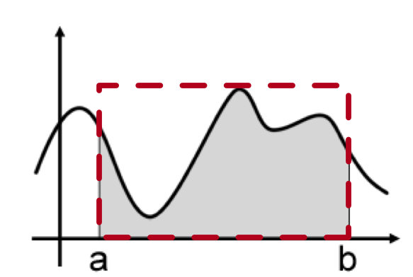
The Monte Carlo “area method” estimates integrals by generating a uniform sample of points and counting how many fall into a planar region
Consider the shaded area as shown below. This is the integral \(I\) which we wish to calculate.

If we choose a point uniformly at random in the rectange (dashed red line) that bounds the shaded area, the probability \(p\) that the point falls in the shaded area is
\[p = \frac{I}{A}\]
where \(A\) is the area of the bounding rectangle. This means that the integral \(I\) can be calculated if we know the area of the bounding rectangle and the probability \(p\):
\[I = Ap\]
To calculate \(p\) we can randomly generate \(N\) points in the bounding area and keep count as to how many lie in the shaded area. If \(k\) lie in the shaded area then the fraction of points \(\frac{k}{N}\) should be equal to the probability \(p\).
\[I = \frac{Ak}{N}\]
We can extend this approach to higher dimensions to consider integrands lying within a bounding volume, or higher dimensional space (which is considered in the extension exercise for this lesson).
We can use the Monte Carlo area method to estimate pi
We’ll now use this approach to give us an estimate for the value of pi by considering the area under a quarter-circle.
The relevant equations are:
square area: \(A_s = (2 r)^2\)
circle area: \(A_c = \pi r^2\)
The ratio of the areas can be related to \(\pi\) through the following expressions:
\[\frac{A_c}{A_s} = \frac{\pi r^2}{4 r^2} = \frac{\pi}{4}\]
\[\pi = 4\frac{A_c}{A_s}\]
To approximate the ratio \(\frac{A_c}{A_s}\) we will generate a (uniform) pseudo-random number between 0 and 1 for our x-coordinates, and a (uniform) pseudo-random number between 0 and 1 for our y-coordinates. We will then check if our random point lies in or out of the circle. The probability \(P_i\) that our point lies in the circle is related to the area ratio and so value of pi:
\[P_i = \frac{A_c}{A_s} = \frac{\pi}{4}\]
The Monte Carlo area method can be translated into Python code
estimate_pi(1000)3.104estimate_pi(2000)3.176This method usually improves with the number of points, however there can be some variation due to the randomness of the numbers used. If you would like others to reproduce your exact results, you can seed the (pseudo-)random number generator:
random.seed(1)
print("error is {}".format(math.pi-estimate_pi(1000)))
error is 0.029592653589793017random.seed(1)
print("error is {}".format(math.pi-estimate_pi(2000)))error is -0.004407346410206792Monte Carlo integration is computationally efficient for particular types of integrand
The error when using Monte Carlo integration is proportional to \(N^{-\frac{1}{2}}\), which is larger than the rectangular slice approach with error order \(h \propto N^{-1}\) (where \(N\) in this case is the number of integration slices). However Monte Carlo methods are more flexible and can be used where other methods break-down: for example, they are particularly useful for integrating functions where the integrand varies very quickly, and/or where the integral is over many variables. In many cases, for “well behaved” functions, an approach based on Riemann summation will give more accurate and computationally efficient results.