import math

def sin(x):

    return math.sin(x)

def rectangular_slice_integral(f_x, a, b, N):

    integral = 0
    h = (b-a) / N   # h is the width of each slice
    for i in range(N):
        x = a + h*i # the x value for the slice
        integral += f_x(x)*h
return integralRiemann sums
Depending on the functional form of f(x), it may not be possible to calculate an integral analytically
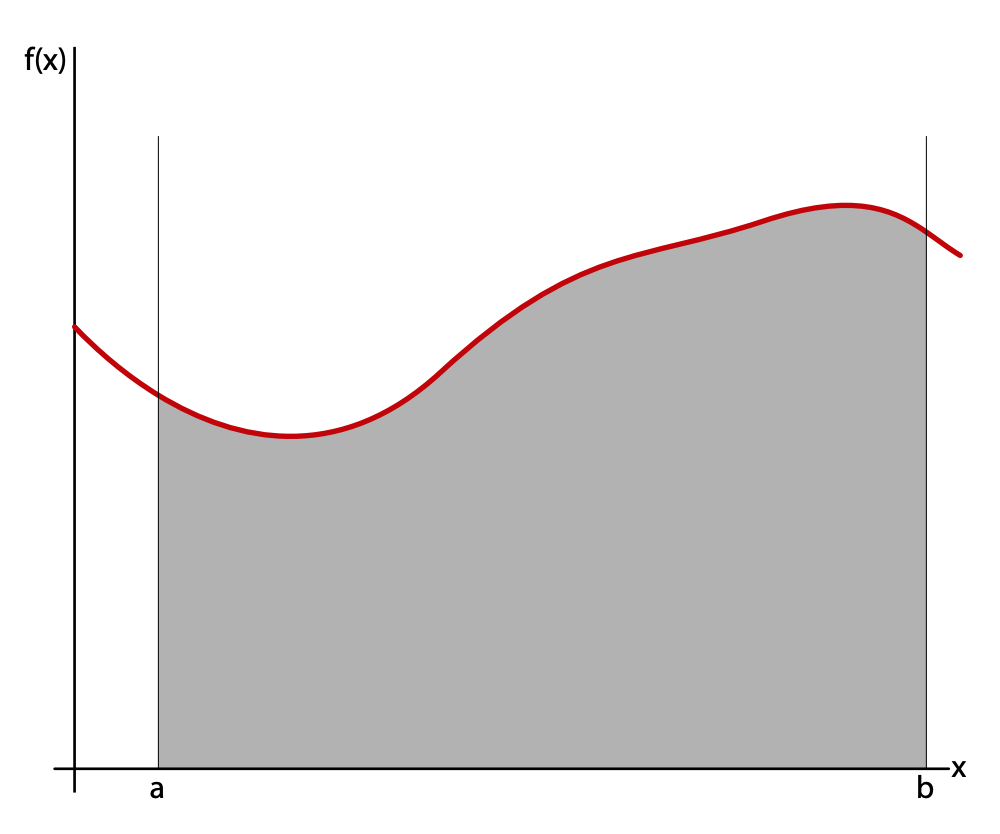
The integral of \(f(x)\) from \(a\) to \(b\) is the area under the curve. Depending on the functional form of \(f(x)\), it may not be possible to calculate the integral analytically.

Riemann sums are a family of methods used for approximating integrals
The Riemann definition of the integral \(I\) is:
\[ I = \lim_{n\to\infty} \sum_{i=1}^N h f(x_i)\]
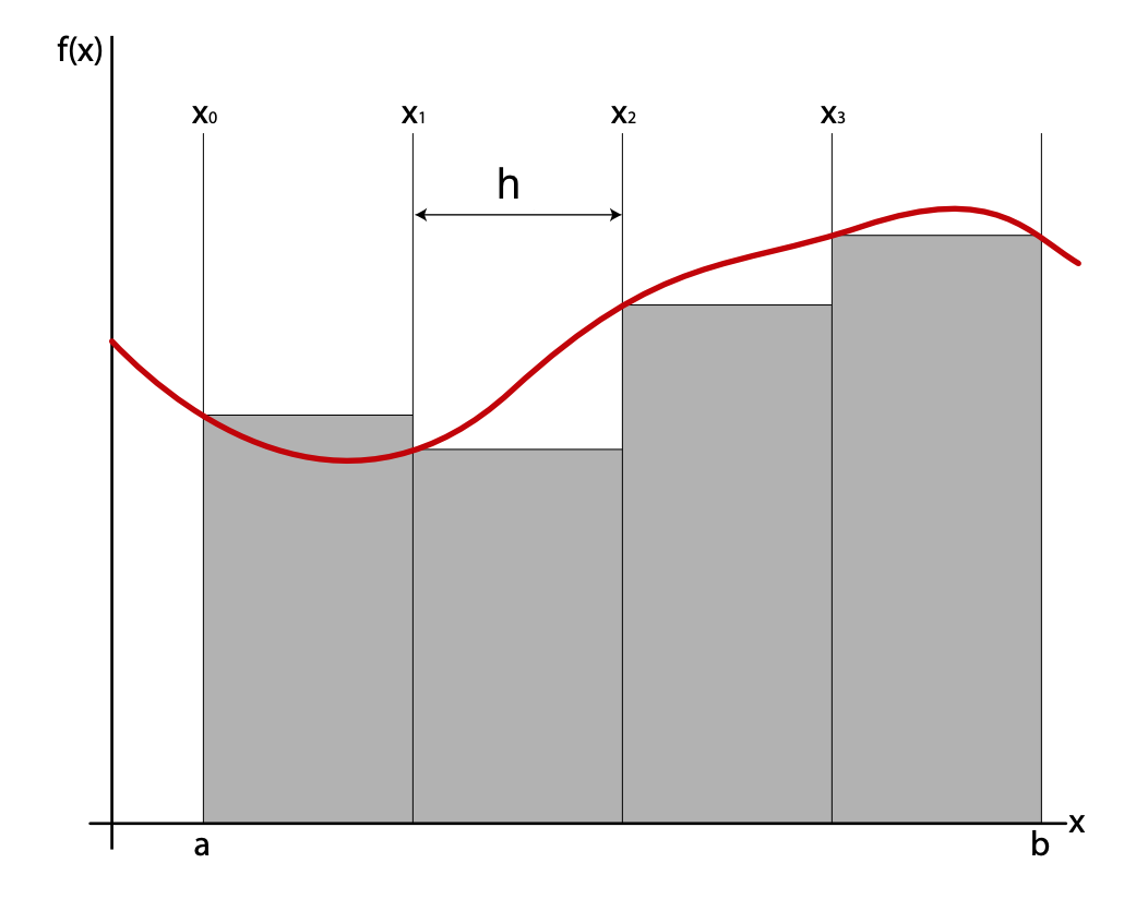
where the domain of integration has been split into \(N\) slices, each with width \(h = \frac{b-a}{N}\). As we cannot in practice consider an infinite number of slices, this definition will give an approximation to the exact answer. By making \(N\) large are approximation will, in many cases, be reasonable.
The simplest Riemann sum is based on rectangular slices
The simplest way to use this approach is to calculate \(f(x_i)\) at some point on each slice and then calculate the area of the associated rectangle:
\[ A_i = hf(x_i)\]
The integral is given by summing over all of the rectangles:
\[ \int_a^b f(x_i) dx \approx \sum_{i=1}^N A_i \]

The rectangular slices method can be translated to Python code in a straight-forward manner
For example, we may want to calculate the integral of \(\sin(x)\) from 0 to \(\frac{\pi}{2}\). This is an integral that can be evaluated analytically, so it doesn’t usually make sense to calculate numerically - however, in this case, we can use it to establish that our method is correct.
Note that the function rectangular_slice_integral has an argument f_x which is itself a function. This is valid Python - you can pass one function to another function as an argument.
rectangular_slice_integral(sin,0,math.pi/2,100)0.9921254566056334In fact, it is possible to pass the math.sin() function directly to rectangular_slice_integral():
rectangular_slice_integral(math.sin,0,math.pi/2,100)0.9921254566056334This is pretty close to the correct value of 1. To improve our approximation we can increase the number of slices:
rectangular_slice_integral(math.sin,0,math.pi/2,200)0.9960678687587687The Riemann sums method a zeroth-order integration rule that will integrate a zeroth-order polynomial (ie, constant number) exactly. It has an error of order \(h\) (\(\mathcal{O}(h)\)) - when we halve the rectangular width, we halve the error.
Riemann sums can be adapted for use with discrete data
Not all integrations are integrations of functions. For example, we may want to integrate experimental data, in which case there is no function to call to find the value of f(x). Instead, the most likely form of f(x) is given by the list of data values. In this case we can use the same method, but the implementation is slightly different:
def rectangular_slice_integral_discrete(data, h):

    return h*sum(data)
Note that this assumes the data is evenly spaced at width \(h\) .
To test our function using the same example as above we need to generate a list of sin(x) values between 0 to \(\frac{\pi}{2}\):
import numpy as np

h = (math.pi/2)/100
sin_0_90 = [math.sin(x) for x in np.arange(0,math.pi/2,h)]
where we are using Python list comprehension and the Numpy arange function to generate a list of evenly spaced floats.
If we are simulating experimental data we should add a little noise or randomness to the data. We can use the Python standard library random and list comprehension to do this:
import random

sin_0_90_noise = [x+random.uniform(-0.1,0.1) for x in sin_0_90]
We can now pass this list to our function rectangular_slice_integral_discrete:
rectangular_slice_integral_discrete(sin_0_90_noise, h)1.0094729791206596We can visualise the exact sinusoidal curve and noisy sinusoidal curve using the matplotlib plotting library:
import matplotlib.pyplot as plt

plt.plot(np.arange(0,math.pi/2,h),sin_0_90,label="exact sine")
plt.plot(np.arange(0,math.pi/2,h),sin_0_90_noise,label="noisy sine")
Higher-order Riemann sums increase the accuracy of our approximations
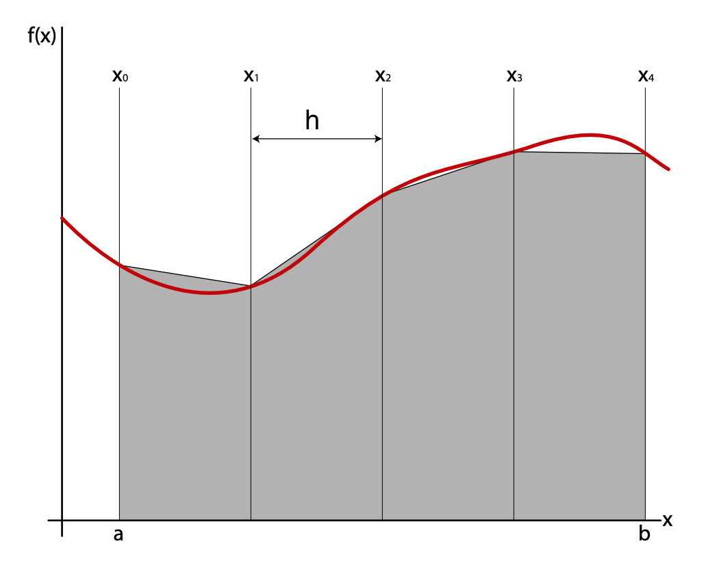
We can greatly improve the efficiency of our integration by approximating the slices as trapezoids instead of as rectangles. This is because the area under the trapezoids is a considerably better approximation to the area under the curve.
The trapezoidal rule a first-order integration rule that will integrate a first-order polynomial (ie, a straight line) exactly. We can say it is accurate to order \(h\) (\(\mathcal{O}(h)\)) and has an error of order \(h^2\) \(\mathcal{O}(h^2)\) .

In many cases we can use Simpson’s Rule for greater accuracy still. This technique involves fitting quadratic curves to pairs of slices and then calculating the area under the quadratics. In many cases Simpson’s rule is more accurate than the trapezoidal rule, but this is not guaranteed for all integrands.