

3. The Atoms Object#
3.1. Overview#
Questions
How can I describe a molecule or crystal using the
Atomsclass?How can I access and adjust
Atomsinformation?What built-in help is available from ASE?
How can I read in a molecule or crystal from a database or external programme?
Objectives
Create and visualise an
AtomsobjectUse
ase.buildto construct common crystal structuresReturn simple structural information from an
AtomsobjectAdjust default properties of an
AtomsobjectRead in a CIF file
Keypoints
Molecules and materials are represented by the
AtomsclassPeriodic boundary conditions are used to simulate an infinitely large system: crystals require
cell(unit cell) andpbc(periodic boundary conditions)Getter methods (
get_positions(),get_masses(), …) retrieve informationSetter methods (
set_cell(),set_initial_magnetic_moments(), …) modify the objectase.io.readandase.io.writehandle 50+ file formats
3.2. Lecture Slides#
The slides for this tutorial are embedded below. 📥 Download slides (.pptx) | Open in full screen
3.3. Molecules and materials are represented by the Atoms class#
The Atoms class is the central data structure in ASE. It holds:
Chemical symbols (or atomic numbers) of each atom
Positions of each atom (in Ångströms)
Optionally: the unit cell, periodic boundary conditions, momenta, charges, magnetic moments, …
To use the Atoms class we need to import it from the ase library:
from ase import Atoms
3.3.1. Creating a simple isolated molecule#
We can define a diatomic (two-atom) molecule by providing lists of symbols and Cartesian positions. Below we assign the Atoms object to the variable N2_molecule (we could have called it anything, but your variable names should always be descriptive).
# N2 molecule
d = 1.10  # N-N bond length in Angstrom
N2_molecule = Atoms(['N', 'N'], positions=[(0., 0., 0.), (0., 0., d)])
Alternatively, we can provide a chemical formula as a string
# Shorthand: chemical formula string
N2_molecule = Atoms('N2', positions=[(0., 0., 0.), (0., 0., d)])
Once we have created the Atoms object we can get stored information:
print(f"Formula: {N2_molecule.get_chemical_formula()}")
print(f"Number of atoms: {len(N2_molecule)}")
Formula: N2
Number of atoms: 2
3.3.2. Visualising an Atoms object#
We can use ase.visualize.view with the nglview backend to display structures inline in a Jupyter notebook.
This will display an interactive 3D view in a Jupyter notebook: Left-click-and-drag to rotate; scroll to zoom.
from ase.visualize import view

view(N2_molecule, viewer='ngl')
If nglview is not installed then we can use matplotlib and ase to produce a non-interative display
import matplotlib.pyplot as plt
from ase.visualize.plot import plot_atoms

fig, ax = plt.subplots()
plot_atoms(N2_molecule, ax, show_unit_cell = 2, radii=0.2, rotation=('30x,0y,0z'))
ax.set_title('N₂ molecule')
ax.axis('off')
plt.tight_layout()
plt.show()
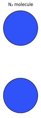
The key function in the code block above is plot_atoms. To understand what optional arguments can be used you can access the in-built help using ?:
plot_atoms?
Signature: plot_atoms(atoms: 'Atoms', ax: 'Axes | None' = None, **kwargs) -> 'Axes'
Docstring:
Plot an Atoms object in a matplotlib subplot.

Axis decorations will always be removed.

For finer control of plot appearance or composition of custom plot
arrangements, consider using plot_atoms_raw() to plot directly to given
Matplotlib Axes.

Parameters
----------
atoms : Atoms object
ax : Matplotlib subplot object
rotation : str, optional
    In degrees. In the form '10x,20y,30z'
show_unit_cell : int, optional, default 2
    Draw the unit cell as dashed lines depending on value:
    0: Don't
    1: Do
    2: Do, making sure cell is visible
radii : float, optional
    The radii of the atoms
colors : list of strings, optional
    Color of the atoms, must be the same length as
    the number of atoms in the atoms object.
scale : float, optional
    Scaling of the plotted atoms and lines.
offset : tuple (float, float), optional
    Offset of the plotted atoms and lines.
File:      ~/miniconda3/envs/kl6003/lib/python3.13/site-packages/ase/visualize/plot.py
Type:      function
3.4. Describing crystals: cell and pbc#
Crystals are described by atomic positions inside a periodic unit cell. Two key keywords:
cell— the unit cell vectors (3×3 matrix, or 3 lengths for cubic cells)pbc— periodic boundary conditions (True/False per direction)
The atomic positions can be specified as an absolute position (positions), or as a fractional position in the unit cell (scaled_positions).
3.4.1. Example: Zinc blende GaN#
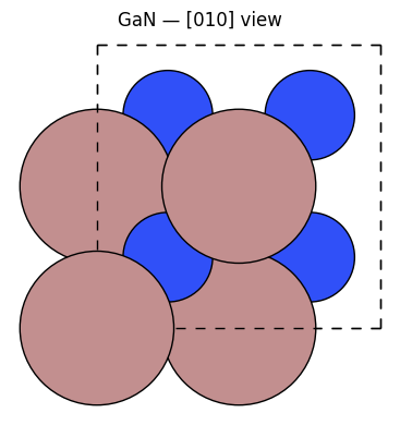
GaN is a wide-bandgap semiconductor widely used in blue LEDs and increasingly explored as a host for single photon emitters. Here we construct the zinc blende polymorph.
import numpy as np
from ase import Atoms

# Zinc blende GaN: a = 4.50 Angstrom
a = 4.50
gan = Atoms('Ga4N4',
            scaled_positions=[
                [0.00, 0.00, 0.00],  # Ga
                [0.00, 0.50, 0.50],  # Ga
                [0.50, 0.00, 0.50],  # Ga
                [0.50, 0.50, 0.00],  # Ga
                [0.25, 0.25, 0.25],  # N
                [0.25, 0.75, 0.75],  # N
                [0.75, 0.25, 0.75],  # N
                [0.75, 0.75, 0.25],  # N
            ],
            cell=[a, a, a],
            pbc=True)

print(f"Formula: {gan.get_chemical_formula()}")
print(f"Number of atoms: {len(gan)}")
print(f"Unit cell (Å):\n{gan.cell}")
Formula: Ga4N4
Number of atoms: 8
Unit cell (Å):
Cell([4.5, 4.5, 4.5])
# Visualise the GaN crystal
from ase.visualize.plot import plot_atoms

fig, axes = plt.subplots(1, 1, figsize=(10, 4))

plot_atoms(gan, axes, rotation=('0x,90y,0z'))
axes.set_title('GaN — [010] view')
axes.axis('off')
plt.tight_layout()
plt.show()
3.5. ase.build — tools for constructing structures#
ASE also provides set of structure-building utilities in ase.build. These are particularly useful for constructing more complex structures such as surfaces.
Function |
Purpose |
|---|---|
|
Common crystal structures (FCC, BCC, diamond, wurtzite, …) |
|
Molecules from the G2 database |
|
Cut surfaces from a bulk structure |
|
Create a supercell with an arbitrary transformation matrix |
from ase.build import bulk

diamond_C  = bulk('C',   'diamond',  a=3.57)
zincblende_GaN = bulk('GaN', 'zincblende', a=4.50)
rocksalt_MgO = bulk('MgO', 'rocksalt', a=4.21)

for name, atoms in [('Diamond C', diamond_C),
                    ('Zincblende GaN', zincblende_GaN),
                    ('Rocksalt MgO', rocksalt_MgO)]:
    print(f"{name}: {atoms.get_chemical_formula()} "
          f"({len(atoms)} atoms, volume = {atoms.get_volume():.2f} ų)")
Diamond C: C2 (2 atoms, volume = 11.37 ų)
Zincblende GaN: GaN (2 atoms, volume = 22.78 ų)
Rocksalt MgO: MgO (2 atoms, volume = 18.65 ų)
3.6. Getter methods#
Remember, once we have an Atoms object, we can retrieve information using getter methods:
print("Positions (Å):")
print(gan.get_positions())

print("\nChemical symbols:")
print(gan.get_chemical_symbols())

print("\nAtomic masses (u):")
print(gan.get_masses())

print("\nCell volume (ų):", gan.get_volume())
Positions (Å):
[[0.    0.    0.   ]
 [0.    2.25  2.25 ]
 [2.25  0.    2.25 ]
 [2.25  2.25  0.   ]
 [1.125 1.125 1.125]
 [1.125 3.375 3.375]
 [3.375 1.125 3.375]
 [3.375 3.375 1.125]]

Chemical symbols:
['Ga', 'Ga', 'Ga', 'Ga', 'N', 'N', 'N', 'N']

Atomic masses (u):
[69.723 69.723 69.723 69.723 14.007 14.007 14.007 14.007]

Cell volume (ų): 91.12499999999999
The positions, chemical symbols and atomic masses are returned as numpy arrays.
print(type(gan.get_positions()))
<class 'numpy.ndarray'>
This means that if we want to return e.g. the position of the first three atoms we can use array slicing:
print(gan.get_positions()[:2])
[[0.   0.   0.  ]
 [0.   2.25 2.25]]
3.7. Setter methods#
We can modify an Atoms object after creation using setter methods. These methods will overwrite the original settings, so if you want to keep the original object you must create an object first:
# Copy the structure and apply a small strain
import copy
strained = gan.copy()

# Biaxial strain in x-y plane (e.g. from epitaxial growth on a substrate)
cell = strained.get_cell()
strain = 0.02  # 2% tensile strain
cell[0] *= (1 + strain)
cell[1] *= (1 + strain)
strained.set_cell(cell, scale_atoms=True)

print(f"Original lattice constant: {gan.cell[0,0]:.4f} Å")
print(f"Strained lattice constant: {strained.cell[0,0]:.4f} Å")

# Magnetic moments — relevant for spin-based quantum systems
gan.set_initial_magnetic_moments([0.0] * len(gan))
print(f"\nInitial magnetic moments: {gan.get_initial_magnetic_moments()}")
Original lattice constant: 4.5000 Å
Strained lattice constant: 4.5900 Å

Initial magnetic moments: [0. 0. 0. 0. 0. 0. 0. 0.]
3.7.1. Exercise: Creating wurtzite#
Construct a wurtzite GaN unit cell (the more common hexagonal polymorph). It has:
Lattice parameters: a = 3.19 Å, c = 5.19 Å
hexagonal cell matrix: \begin{pmatrix} a & 0 & 0 \ -\frac{a}{2} & \frac{a\sqrt{3}}{2} & 0 \ 0 & 0 & c \end{pmatrix}
Scaled positions: Ga at (1/3, 2/3, 0) and (2/3, 1/3, 1/2); N at (1/3, 2/3, 3/8) and (2/3, 1/3, 7/8)
Use ase.build.bulk('GaN', crystalstructure='wurtzite', a=3.19, c=5.19) to check your answer.
3.7.2. Exercise: Creating diamond#
The NV centre in diamond consists of a nitrogen substitutional adjacent to a carbon vacancy. Build a diamond cubic unit cell (a = 3.57 Å, 8 atoms) and print the nearest-neighbour C-C bond length. Compare to the known value of 1.54 Å.
For this question you need to find the atomic positions in the diamond structure, and may want to use the ASE documentation to find a function for finding nearest neighbour distances.
3.8. Writing and Reading structures with ase.io.read#
ASE can read and write over 50 crystal structure file formats.
The primary function to read in structures is ase.io.read, which auto-detects the format from the file extension.
Common formats you might encounter:
Format |
Extension |
Used by |
|---|---|---|
CIF |
|
Crystallographic databases (ICSD, Materials Project) |
XYZ |
|
General |
extXYZ |
|
many ML codes |
Trajectory |
|
ASE native format |
3.8.1. Build a structure using ASE’s build module#
import ase.io
from ase.io import read, write
from ase import Atoms
import numpy as np

from ase.build import bulk

gan_wz = bulk('GaN', crystalstructure='wurtzite', a=3.19, c=5.19)
print(f"Wurtzite GaN: {len(gan_wz)} atoms, formula {gan_wz.get_chemical_formula()}")
print(f"Cell (Å):\n{gan_wz.cell}\n")    # \n creates newlines for neater display
Wurtzite GaN: 4 atoms, formula Ga2N2
Cell (Å):
Cell([[3.19, 0.0, 0.0], [-1.595, 2.7626210380723593, 0.0], [0.0, 0.0, 5.19]])
3.8.2. Writing to different formats#
import os

# Write to XYZ (a widely used file format)
write('/tmp/GaN_wurtzite.xyz', gan_wz)

# Write to CIF (another widely used file format(
write('/tmp/GaN_wurtzite.cif', gan_wz, format='cif')
3.8.3. Inspecting file content#
The extended XYZ format is particularly useful because it stores cell and PBC information in the header line:
with open('/tmp/GaN_wurtzite.xyz') as f:
    print(f.read())
4
Lattice="3.19 0.0 0.0 -1.595 2.7626210380723593 0.0 0.0 0.0 5.19" Properties=species:S:1:pos:R:3 pbc="T T T"
Ga       0.00000000       0.00000000       0.00000000
N       -0.00000000       1.84174736       0.64392903
Ga      -0.00000000       1.84174736       2.59500000
N        0.00000000       0.00000000       3.23892903
Inspecting the cif file shows that it stores the same information in a slightly different format:
with open('/tmp/GaN_wurtzite.cif') as f:
    print(f.read())
data_image0
_chemical_formula_structural       GaNGaN
_chemical_formula_sum              "Ga2 N2"
_cell_length_a       3.19
_cell_length_b       3.19
_cell_length_c       5.19
_cell_angle_alpha    90.0
_cell_angle_beta     90.0
_cell_angle_gamma    120.00000000000001

_space_group_name_H-M_alt    "P 1"
_space_group_IT_number       1

loop_
  _space_group_symop_operation_xyz
  'x, y, z'

loop_
  _atom_site_type_symbol
  _atom_site_label
  _atom_site_symmetry_multiplicity
  _atom_site_fract_x
  _atom_site_fract_y
  _atom_site_fract_z
  _atom_site_occupancy
  Ga  Ga1       1.0  0.0  0.0  0.0  1.0000
  N   N1        1.0  0.3333333333333333  0.6666666666666666  0.12407110408213018  1.0000
  Ga  Ga2       1.0  0.3333333333333333  0.6666666666666666  0.5  1.0000
  N   N2        1.0  0.0  0.0  0.6240711040821302  1.0000
Read back in the XYZ file and show that it matches the positions
gan_readback = read('/tmp/GaN_wurtzite.xyz')
print("Read back from XYZ:")
print(f"  Formula: {gan_readback.get_chemical_formula()}")
print(f"  Positions match: {np.allclose(gan_wz.positions, gan_readback.positions)}")
Read back from XYZ:
  Formula: Ga2N2
  Positions match: True
3.8.4. Exercise: hBN structure#
Download the CIF file for hexagonal boron nitride (hBN) from the The Materials Project. Read it with ASE and print the lattice parameters and number of atoms in the unit cell.