Questions:
- Which physical systems can be described using a PDE?
- What is the Laplacian operator?
- When to I need boundary conditions and initial conditions?
In the previous section of the course we studied
ordinary differential equations . ODEs have a single input (also known as independent variable) - for example, time.Partial differential equations (PDEs) have multiple inputs (independent variables). For example, think about a sheet of metal that has been heated unevenly across the surface. Over time, heat will diffuse through the 2-dimensional sheet. The temperature depends on both time and position - there are two inputs.
Because PDEs have multiple inputs they are generally much more difficult to solve analytically than ODEs. However, there are a range of numerical methods that can be used to find approximate solutions.
PDEs have application across a wide variety of topics
The same type of PDE often appears in different contexts. For example, the diffusion equation takes the form:
\begin{equation} \nabla^2T = \alpha \frac{\partial T}{\partial t} \end{equation}When used to describe heat diffusion, this PDE is known as the heat equation. This same PDE however can be used to model other seemingly unrelated processes such as brownian motion, or used in financial modelling via the Black-Sholes equation.
Another type of PDE is known as Poisson's equation:
\begin{equation} \nabla^2\phi = f(x,y,z) \end{equation}Poisson's equation can be used to describe electrostatic forces, where $\phi$ is the electric potential. It can also be applied to mechanics (where $\phi$ is the gravitational potential) or thermodynamics (where $\phi$ is the temperature). When $f(x,y,z)=0$ this equation is known as Laplace's equation.
The third common type of PDE is the wave equation:
\begin{equation} \nabla^2r = \alpha \frac{\partial^2 r}{\partial t^2} \end{equation}This describes mechanical processes such as the vibration of a string or the motion of a pendulum. It can also be used in electrodynamics to describe the exchange of energy between the electric and magnetic fields.
The Laplacian operator corresponds to an average rate of change
But what is the operator $\nabla^2$?. This is the Laplacian operator. When applied to $\phi$ and written in full for a three dimensional cartesian coordinate system with dependent variables $x$, $y$ and $z$ it takes the following form:
\begin{equation} \nabla^2\phi = \frac{\partial^2\phi}{\partial x^2} + \frac{\partial^2\phi}{\partial y^2} + \frac{\partial^2\phi}{\partial z^2}. \end{equation}We can think of the laplacian as encoding an average rate of change - the difference between a value at a point and the average of the values around that point.
youtube_video("https://youtu.be/EW08rD-GFh0").display()
Boundary value problems
Boundary value problems describe the behaviour of a variable in a space and we are given some constraints on the variable around the boundary of that space. For example, consider the 2-dimensional problem of a thin rectangular sheet with one side at voltage $V$ and all others at voltage zero.
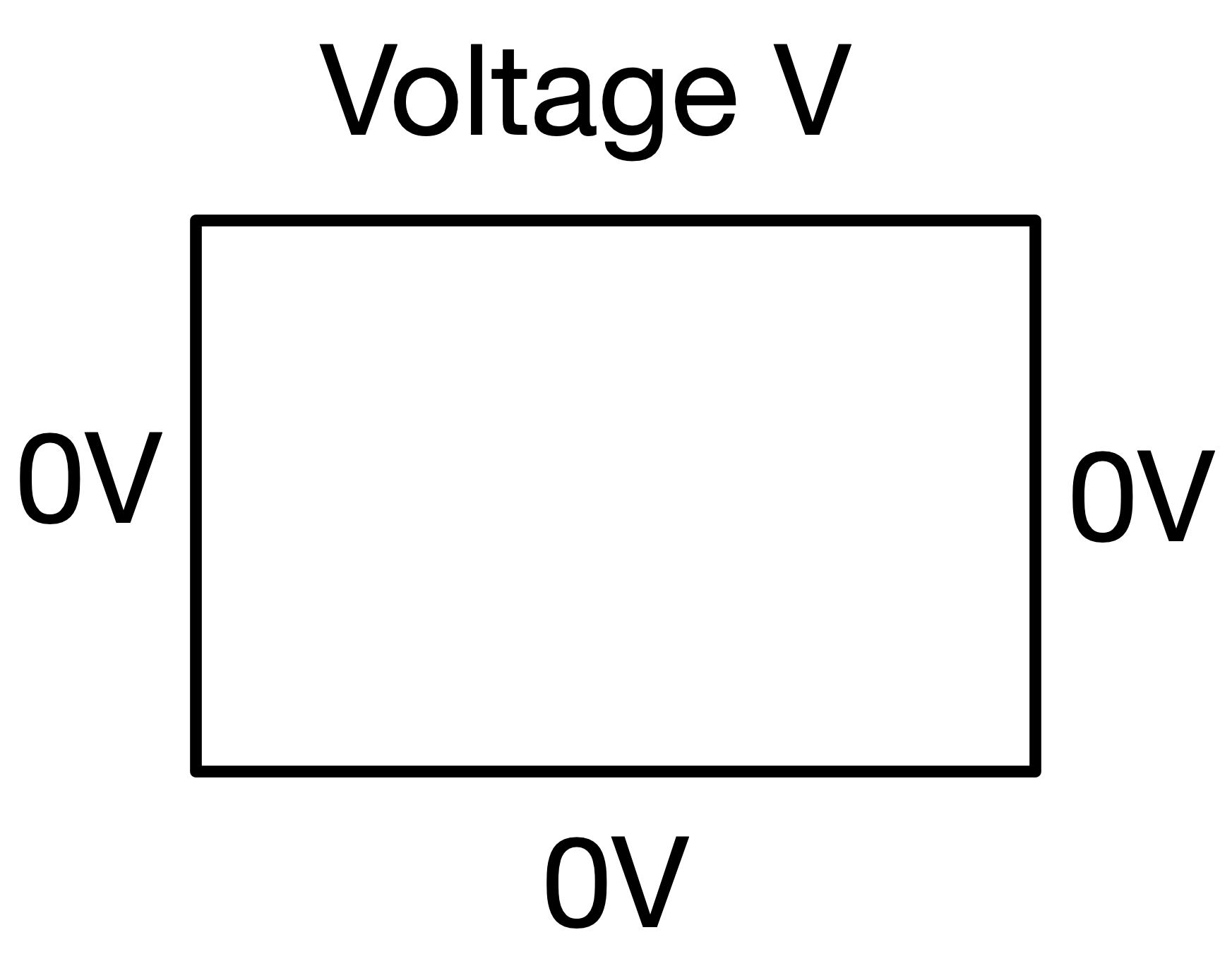
The specification that one side is at voltage $V$ and all others are at voltage zero are the boundary conditions. We could then calculate the electrostatic potential $\phi$ at all points within the sheet using the two-dimensional Laplace's equation:
\begin{equation} \nabla^2\phi = \frac{\partial^2\phi}{\partial x^2} + \frac{\partial^2\phi}{\partial y^2} = 0 \end{equation}Initial value problems
Initial value problems are where the field - or other variable of interest - is varying in both space and time. We now require boundary conditions and initial values. This is a more difficult type of PDE to solve.
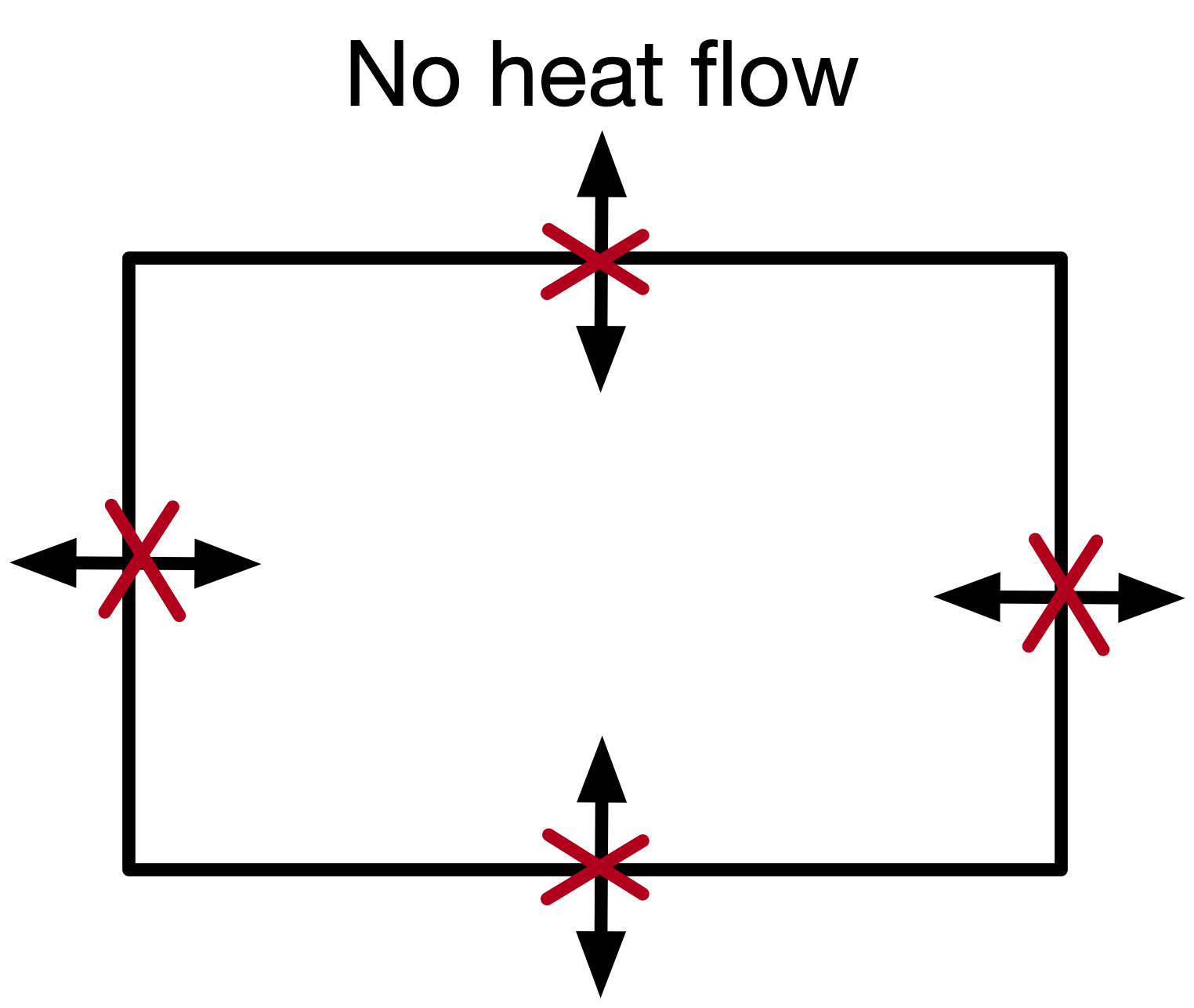
For example, consider heat diffusion in a two-dimensional sheet. Here we could specify that there is no heat flow in or out of the sheet - this is the boundary condition.
We could also specify that at time $t=0$ the centre of the sheet is at temperature $T_1$, whilst surrounding areas are at temperature $T_0$. This is the initial condition. It differs from a boundary condition in that we are told what the temperature is at the start of our time grid (at $t=0$) but not at the end of our time grid (when the simulation finishes).
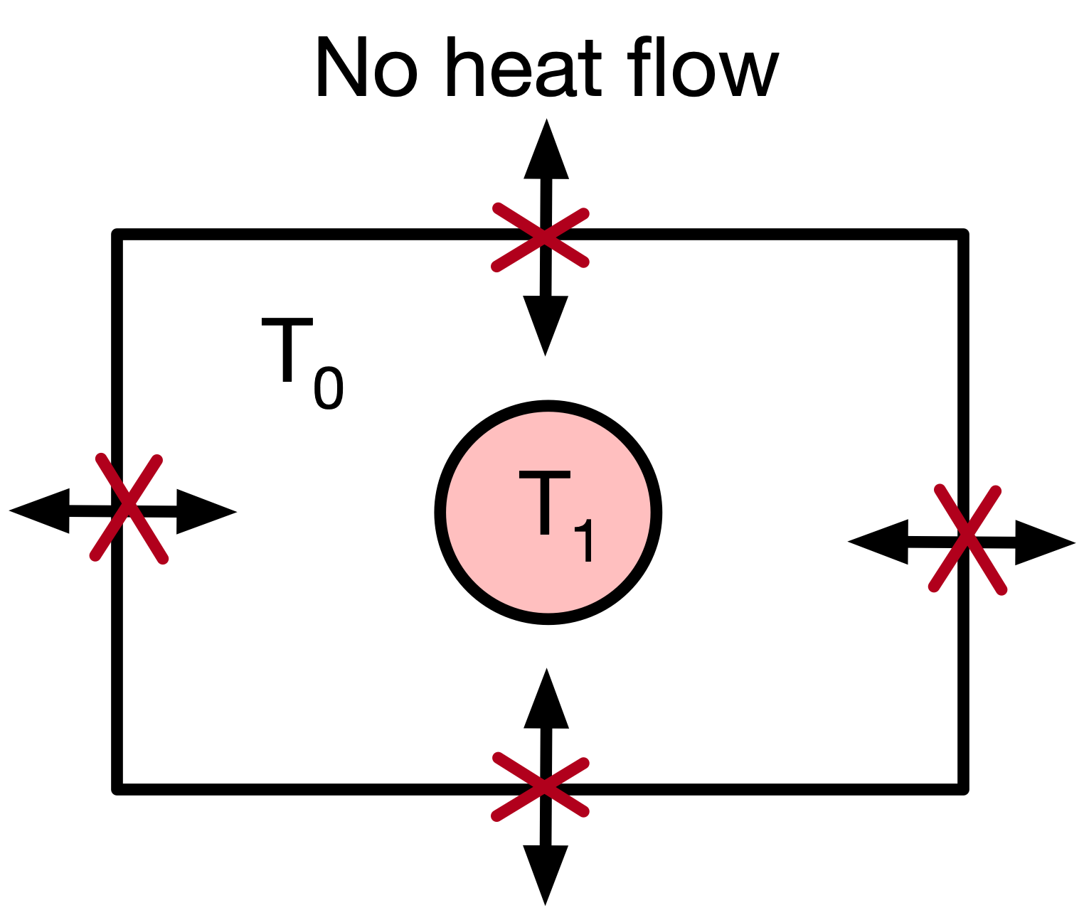
We could then calculate the temperature at time $t$ at all points $[x,y]$ within the sheet using the two-dimensional Diffusion equation:
\begin{equation} \nabla^2T = \frac{\partial^2 T}{\partial x^2} + \frac{\partial^2 T}{\partial y^2}=\alpha \frac{\partial T}{\partial t} \end{equation}Laplace's equation for electrostatics
Questions:
- How do I use a finite difference method to calculate derivatives?
- How do I use the relaxation method to solve Laplace's equation?
The method of finite differences
Consider the two-dimensional Laplace equation for the electric potential $\phi$ subject to appropriate boundary conditions:
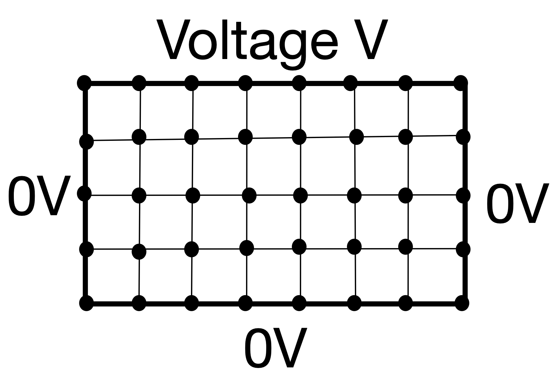
\begin{equation} \frac{\partial^2\phi}{\partial x^2} + \frac{\partial^2\phi}{\partial y^2} = 0 \end{equation}The method of finite differences involves dividing the space into a grid of discrete points $[x,y]$ and calculating numerical derivatives or at each of these points.
But how do we calculate these numerical derivatives?
Real physical problems are in three dimensions, but we can more easily visualise the method of finite differences - and the extension to three dimensions is straight forward.
Calculating numerical derivatives
The standard definition of a derivative is
\begin{equation} \frac{\mathrm{d} f}{\mathrm{d} x} = \lim_{h\to0}\frac{f(x+h)-f(x)}{h}. \end{equation}To calculate the derivative numerically we make $h$ very small and calculate
\begin{equation} \frac{\mathrm{d} f}{\mathrm{d} x} \simeq \frac{f(x+h)-f(x)}{h}. \end{equation}This is the forward difference because it is measured in the forward direction from $x$.
The backward difference is measured in the backward direction from $x$:
\begin{equation} \frac{\mathrm{d} f}{\mathrm{d} x} \simeq \frac{f(x)-f(x-h)}{h}, \end{equation}and the central difference uses both the forwards and backwards directions around $x$:
\begin{equation} \frac{\mathrm{d} f}{\mathrm{d} x} \simeq \frac{f(x+\frac{h}{h2})-f(x-\frac{h}{2})}{h}, \end{equation}Numerical second-order derivatives
The second derivative is a derivative of a derivative, and so we can calculate it be applying the first derivative formulas twice. The resulting expression (after application of central differences) is:
\begin{equation} \frac{\mathrm{d} ^2f}{\mathrm{d} x^2} \simeq \frac{f(x+h)-2f(x)+f(x-h)}{h^2}. \end{equation}Numerical partial derivatives
The extension to partial derivatives is straight-forward:
\begin{equation} \frac{\mathrm{d} f}{\mathrm{d} x} \simeq \frac{f(x+\frac{h}{h2})-f(x-\frac{h}{2})}{h}, \end{equation}\begin{equation} \frac{\partial f}{\partial x} \simeq \frac{f(x+\frac{h}{2},y)-f(x-\frac{h}{2},y)}{h}, \end{equation}\begin{equation} \frac{\partial f}{\partial y} \simeq \frac{f(x,y+\frac{h}{2})-f(x,y-\frac{h}{2})}{h}, \end{equation}By adding the two equations above, the Laplacian in two dimensions is:
\begin{equation} \frac{\partial ^2f}{\partial x^2} + \frac{\partial ^2f}{\partial y^2} \simeq \frac{f(x+h,y)+f(x-h,y)+f(x,y+h)+f(x,y-h)-4f(x,y)}{h^2}, \end{equation}PDEs --> linear simulatenous equations
Returning to our Laplace equation for for the electric potential $\phi$:
\begin{equation} \frac{\partial^2\phi}{\partial x^2} + \frac{\partial^2\phi}{\partial y^2} = 0 \end{equation}
The numerical Laplacian can be substituted into the equation above, giving us a set of $n$ simulatenous equations for the $n$ grid points.
\begin{equation} \frac{\phi(x+h,y)+\phi(x-h,y)+\phi(x,y+h)+\phi(x,y-h)-4\phi(x,y)}{a^2} = 0, \end{equation}where $a$ is the distance between each grid point.
To solve we use the relaxation method
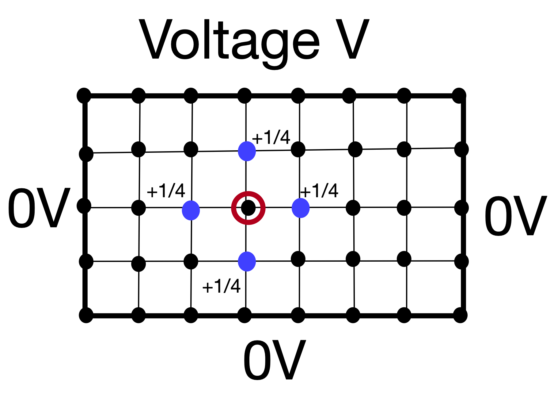
\begin{equation} \frac{\phi(x+h,y)+\phi(x-h,y)+\phi(x,y+h)+\phi(x,y-h)-4\phi(x,y)}{a^2} = 0, \end{equation}\begin{equation} \phi(x,y)=\frac{1}{4}\left(\phi(x+h,y)+\phi(x-h,y)+\phi(x,y+h)+\phi(x,y-h)\right). \end{equation}This tells us that $\phi(x,y)$ is the average of the surrounding grid points, which can be represented visually as:
To solve we use the relaxation method
Step one
Fix $\phi(x,y)$ at the boundaries using the boundary conditions.
Step two
Guess the initial values of the interior $\phi(x,y)$ points - our guesses do not need to be good, and can be zero.
Step three
Calculate new values of $\phi'(x,y)$ at all points in space using an iterative method: \begin{equation} \phi'(x,y)=\frac{1}{4}\left(\phi(x+h,y)+\phi(x-h,y)+\phi(x,y+h)+\phi(x,y-h)\right). \end{equation}
Step four
Repeat until the $\phi(x,y)$ values converge*, and that is our solution.
*Convergence can be tested by specifying what the maximum difference should be between iterations. For example, that $\phi'(x,y)-\phi(x,y)< 1e-5$ for all grid points.
Heat Diffusion
Questions:
- How do I use the Forward-Time Centred-Space method (FTCS) to solve the diffusion equation?
The diffusion equation is an initial value problem
An initial value problem is more complex than a boundary value problem as we are told the starting conditions and then have to predict future behaviour as a function of time.
Example
A 10cm rod of stainless steel initially at a uniform temperature of 20$^\mathrm{o}$ Celsius. The rod is dipped in a hot water bath at 90$^\mathrm{o}$ Celsius at one end, and held in someone's hand at the other. Assume that the hand is at constant body temperature throughout (27$^\mathrm{o}$ Celsius).
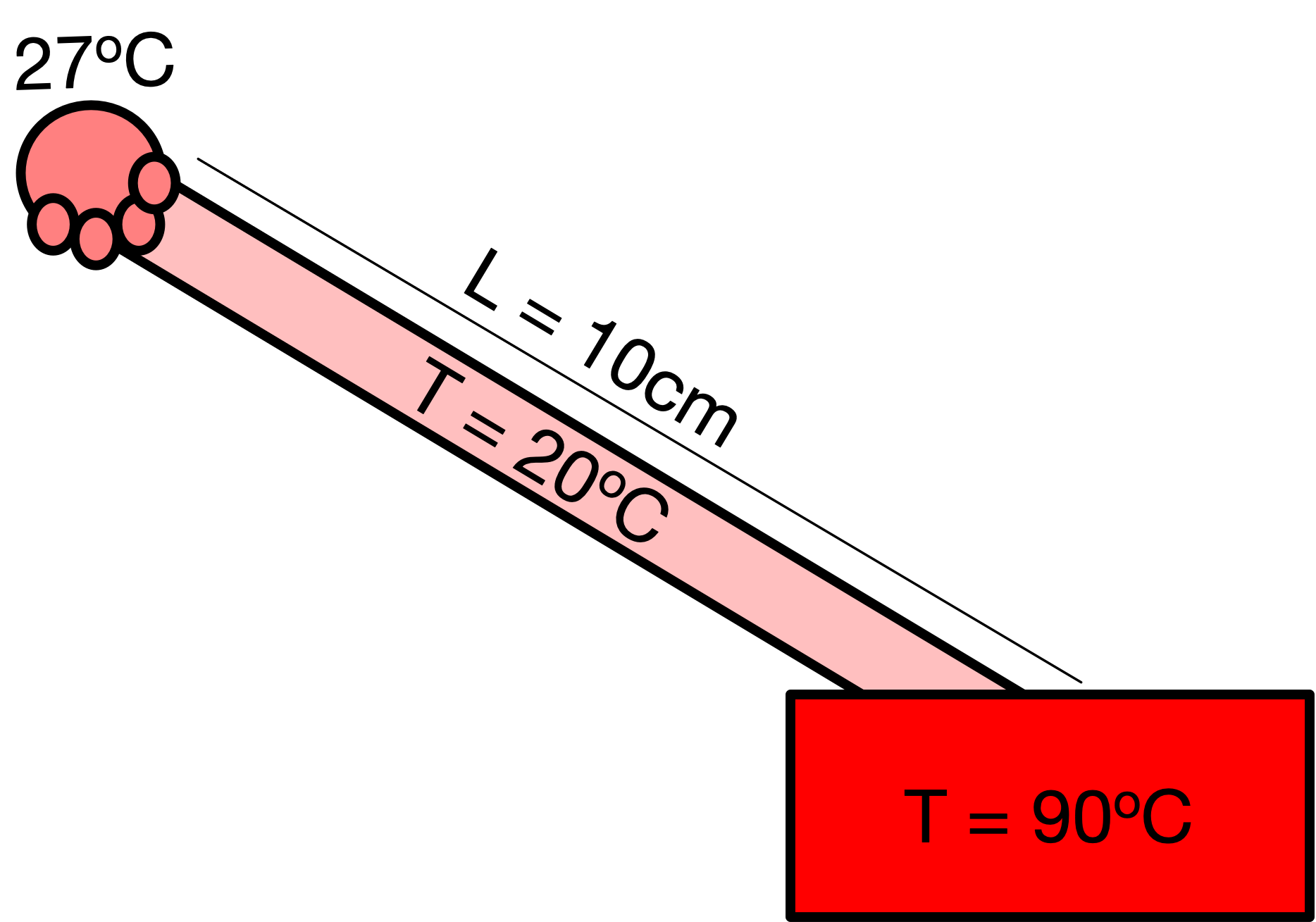
Assume:
- that the rod is perfectly insulated so that heat only moves horizontally --> a 1D problem
- neither the hot water bath or the hand change temperature
Thermal conduction is described by the diffusion equation:
\begin{equation} \frac{\partial \phi}{\partial t} = D\frac{\partial^2 \phi}{\partial x^2}, \end{equation}where $D$ is the material dependent thermal diffusivity. For steel $D=4.25\times10^{-6}\mathrm{m}^2\mathrm{s}^{-1}$.
Why can't we use the relaxation method?
We solved Laplace's equation and that had three variables ($x$,$y$,$z$) - why not do the same thing here?
The problem is that we only have an initial condition in the time dimension - we know the value of $\phi(x,t)$ at $t=0$ but we do not typically know the value of $t$ at a later point. In the spatial dimensions we know the boundary conditions at either end of the grid.
Instead, we will use the Forward-Time Centred-Space method (FTCS).
There are two steps to the Forward-Time Centred-Space method
Step one
Use the finite difference method to express the 1D Laplacian as a set of simulatenous equations:
\begin{equation} \frac{\partial^2\phi}{\partial x^2} = \frac{\phi(x+a,t)+\phi(x-a,t) - 2\phi(x,t)}{a^2} \end{equation}where $a$ is the grid spacing.
Substitute this back into the diffusion equation:
\begin{equation} \frac{d \phi}{d t} = \frac{D}{a^2}(\phi(x+a,t)+\phi(x-a,t)-2\phi(x,t)) \end{equation}We now have a set of simultaneous ODEs for $\phi(x,t)$.
Step two
So we can use Euler's method to evolve the system forward in time. Euler's method for solving an ODE of the form $\frac{d\phi}{dt} = f(\phi,t)$ has the general form:
\begin{equation} \phi(t+h) \simeq \phi(t) + hf(\phi, t). \end{equation}Applying this to Equation 3 gives:
\begin{equation} \phi(x,t+h) = \phi(x,t) + h\frac{D}{a^2}(\phi(x+a,t)+\phi(x-a,t)-2\phi(x,t)) \end{equation}Evaluating numerical errors and accuracy
Questions:
- Which numerical errors are unavoidable in a Python programme?
- How do I choose the optimum step size $h$ when using the finite difference method?
- What do the terms first-order accurate and second-order accurate mean?
- How can I measure the speed of my code?
Finite difference methods have two sources of error
- There are two sources of errors for finite difference methods:
- the approximation that the step size $h$ is small but not zero.
- the numerical rounding errors for floating point numbers
- If we decrease the step size $h$:
- the finite-difference approximation will improve
- the runtime of the programme will increase
- counter-intuitively, the rounding error might increase.
- So it is possible that by decreasing $h$ we make our programme less accurate and it takes longer to run!
To demonstrate this, consider the Taylor expansion of $f(x)$ about $x$:
\begin{equation} f(x+h) = f(x) + hf'(x) +\frac{1}{2}h^2f''(x) + \ldots \end{equation}Re-arrange the expression to get the expression for the forward difference method:
\begin{equation} f'(x) = \frac{f(x+h)}{h} - \frac{1}{2}hf''(x)+\ldots \end{equation}A computer can typically store a number $f(x)$ to an accuracy of 16 significant figures, or $Cf(x)$ where $C=10^{-16}$. In the worst case, this makes the error $\epsilon$ on our derivative:
\begin{equation} \epsilon = \frac{2C|f(x)|}{h} + \frac{1}{2}h|f''(x)|. \end{equation}We want to find the value of $h$ which minimises this error so we differentiate with respect to $h$ and set the result equal to zero.
\begin{equation} -\frac{2C|f(x)|}{h^2} + h|f''(x)| = 0 \end{equation}\begin{equation} h = \sqrt{4C\lvert\frac{f(x)}{f''(x)}\rvert} \end{equation}If $f(x)$ and $f''(x)$ are order 1, then $h$ should be order $\sqrt{C}$, or $10^{-8}$.
Similar reasoning applied to the central difference formula suggests that the optimum step size for this method is $10^{-5}$.