💃 Classifying differential equations 💃¶

Questions:

What is a differential equation?
What is the difference between an ordinary (ODE) and partial (PDE) differential equation?
How do I classify the different types of differential equations?

Objectives:

Identify the dependent and independent variables in a differential equation
Distinguish between and ODE and PDE
Identify the order of a differential equation
Distinguish between linear and non-linear equations
Distinguish between heterogeneous and homogeneous equations
Identify a separable equation

A differential equation is an equation that relates one or more functions and their derivatives¶

The functions usually represent physical quantities (e.g. $\mathbf{F}$))
The derivative represents a rate of change (e.g. acceleration)
The differential equation represents the relationship between the two.
For example, Newton's second law for $n$ particles of mass $m$:

\begin{equation} \mathbf{F}(t,\mathbf{x},\mathbf{v}) = m\frac{d\mathbf{v}}{dt} \end{equation}

An independent variable is... a quantity that varies independently...¶

An independent variable does not depend on other variables
A dependent variable depends on the independent variable

\begin{equation} \mathbf{F}(t,\mathbf{x},\mathbf{v}) = m\frac{d\mathbf{v}}{dt} \end{equation}

$t$ is an independent variable
$x$ and $v$ are dependent variables
Writing $x = x(t)$ makes this relationship clear.

Differential equations can be classified in a variety of ways¶

There are several ways to describe and classify differential equations. There are standard solution methods for each type, so it is useful to understand the classifications.

Once you can cook a single piece of spaghetti, you can cook all pieces of spaghetti!

An ODE contains differentials with respect to only one variable¶

For example, the following equations are ODEs:

\begin{equation} \frac{d x}{d t} = at \end{equation}\begin{equation} \frac{d^3 x}{d t^3} + \frac{x}{t} = b \end{equation}

As in each case the differentials are with respect to the single variable $t$.

Partial differential equations (PDE) contain differentials with respect to several independent variables.¶

An example of a PDE is:

\begin{equation} \frac{\partial x}{\partial t} = \frac{\partial x}{\partial y} \end{equation}

As there is one differential with respect to $t$ and one differential with respect to $y$.

Note also the difference in notation - for ODEs we use $d$ whilst for PDEs we use $\partial$.

The order of a differential equation is the highest order of any differential contained in it.¶

For example:

$\frac{d x}{d t} = at$ is first order.

$\frac{d^3 x}{d t^3} + \frac{x}{t} = b$ is third order.

Note: $\frac{d^3 x}{d t^3}$ does not equal $\left(\frac{d x}{d t}\right)^3$!

Linear equations do not contain higher powers of either the dependent variable or its differentials¶

For example:

$\frac{d^3 x}{d t^3} = at$ and $\frac{\partial x}{\partial t} = \frac{\partial x}{\partial y} $ are linear.

$(\frac{d x}{d t})^3 = at$ and $\frac{d^3 x}{d t^3} = x^2$ are non-linear.

Non-linear equations can be particularly nasty to solve analytically, and so are often tackled numerically.

Homogeneous equations do not contain any non-differential terms¶

For example:

$\frac{\partial x}{\partial t} = \frac{\partial x}{\partial y}$ is a homogeneous equation.

$\frac{\partial x}{\partial t} - \frac{\partial x}{\partial y}=a$ is a heterogeneous equation (unless $a=0$!).

Separable equations can be written as a product of two functions of different variables¶

A separable differential equation takes the form

\begin{equation} f(x)\frac{d x}{d t} = g(t) \end{equation}

Separable equations are some of the easiest to solve as we can split the equation into two independent parts with fewer variables, and solve each in turn - we will see an example of this in the next tutorial.

Keypoints:

An independent variable is a quantity that varies independently
Differential equations can be classified in a variety of ways
An ODE contains differentials with respect to only one variable
The order is the highest order of any differential contained in it
Linear equations do not contain higher powers of either the dependent variable or its differentials
Homogeneous equations do not contain any non-differential terms

Radioactive Decay¶

Questions:

How can I describe radioactive decay using a first-order ODE?
What are initial conditions and why are they important?

Objectives:

Map between physical notation for a particular problem and the more general notation for all differential equations
Solve a linear, first order, separable ODE using integration
Understand the physical importance of initial conditions

Radioactive decay can be modelled a linear, first-order ODE¶

As our first example of an ODE we will model radioactive decay using a differential equation.

We know that the decay rate is proportional to the number of atoms present. Mathematically, this relationship can be expressed as:

\begin{equation} \frac{d N}{d t} = -\lambda N \end{equation}

Note that we could choose to use different variables, for example:

\begin{equation} \frac{d y}{d x} = cy \end{equation}

However we try to use variables connected to the context of the problem. For example $N$ for the Number of atoms.

If we know that 10% of atoms will decay per second we could write:

\begin{equation} \frac{d N}{d t} = -0.1 N \end{equation}

where $N$ is the number of atoms and $t$ is time measured in seconds.

This equation is linear and first-order.

physical notation	generic notation $\left(\frac{dy}{dx} = f(y)\right)$
number of atoms $N$	dependent variable $y$
time $t$	independent variable $x$
decay rate $\frac{dN}{dt}$	differential $\frac{dy}{dx}$
constant of proportionality $\lambda=0.1 $	parameter(s)

The equation for radioactive decay is separable and has an analytic solution¶

The radioactive decay equation is separable:

\begin{equation} \frac{1}{N}\frac{d N}{d t} = -\lambda \end{equation}\begin{equation} \frac{dN}{N} = -\lambda dt. \end{equation}

We can then integrate each side:

\begin{equation} \ln N = -\lambda t + const. \end{equation}

and solve for N:

\begin{equation} N = e^{-\lambda t}e^{\textrm{const.}} \end{equation}

To model a physical system an initial value has to be provided¶

\begin{equation} N(t) = e^{-\lambda t}e^{\textrm{const.}} \end{equation}

At the beginning (when $t=0$):

\begin{equation} N (t_0) = e^{0}e^{\textrm{const.}} = e^{\textrm{const.}} \end{equation}

So we can identify $e^{\textrm{const.}}$ as the amount of radioactive material that was present in the beginning. We denote this starting amount as $N_0$.

Substituting this back into Equation 4, the final solution can be more meaningfully written as:

\begin{equation} N = N_0 e^{-\lambda t} \end{equation}

We now have not just one solution, but a whole class of solutions that are dependent on the initial amount of radioactive material $N_0$.

Remember that not all mathematical solutions make physical sense. To model a physical system, this initial value (also known as initial condition) has to be provided alongside the constant of proportionality $\lambda$.

ODEs can have initial values or boundary values¶

ODEs have either initial values or boundary values. Take Newton's second law as an example:

\begin{equation} \frac{\mathrm{d}^2x}{\mathrm{d}t^2} = -g \end{equation}

An initial value problem would be where we know the starting position and velocity. A boundary value problem would be where we specify the position of the ball at times $t=t_0$ and $t=t_1$.

For second-order ODEs (such as acceleration under gravity) we need to provide two initial/boundary conditions, for third-order ODEs we would need to provide three, and so on. Our radioactive decay example was a first-order ODE and so we only had to provide a single initial condition.

Keypoints:

Radioactive decay can be modelled a linear, first-order ODE
The equation for radioactive decay is separable and has an analytic solution
To model a physical system an initial value has to be provided
The number of initial conditions depends on the order of the differential equation

Euler's Method¶

Questions:

How do I use Euler's method to solve a first-order ODE?

Objectives:

Use Euler's method, implemented in Python, to solve a first-order ODE
Understand that this method is approximate and the significance of step size $h$
Compare results at different levels of approximation using the matplotlib library.

There are a variety of ways to solve an ODE¶

In the previous lesson we considered nuclear decay:

\begin{equation} \frac{\mathrm{d} N}{\mathrm{d} t} = -\lambda N \end{equation}

This is one of the simplest examples of am ODE - a first-order, linear, separable differential equation with one dependent variable. We saw that we could model the number of atoms $N$ by finding an analytic solution through integration:

\begin{equation} N = N_0 e^{-\lambda t} \end{equation}

However there is more than one way to crack an egg (or solve a differential equation). We could have, instead, used an approximate, numerical method. One such method - Euler's method - is this subject of this lesson.

A function can be approximated using a Taylor expansion¶

The Taylor series is a polynomial expansion of a function about a point. For example, the image below shows $\mathrm{sin}(x)$ and its Taylor approximation by polynomials of degree 1, 3, 5, 7, 9, 11, and 13 at $x = 0$.

Credit: Image By IkamusumeFan - CC BY-SA 3.0, Commons Wikimedia

The Taylor series of $f(x)$ evaluated at point $a$ can be expressed as:

\begin{equation} f(x) = f(a) + \frac{\mathrm{d} f}{\mathrm{d} x}(x-a) + \frac{1}{2!} \frac{\mathrm{d} ^2f}{\mathrm{d} x^2}(x-a)^2 + \frac{1}{3!} \frac{\mathrm{d} ^3f}{\mathrm{d} x^3}(x-a)^3 \end{equation}

Returning to our example of nuclear decay, we can use a Taylor expansion to write the value of $N$ a short interval $h$ later:

\begin{equation} N(t+h) = N(t) + h\frac{\mathrm{d}N}{\mathrm{d}t} + \frac{1}{2}h^2\frac{\mathrm{d}^2N}{\mathrm{d}t^2} + \ldots \end{equation}\begin{equation} N(t+h) = N(t) + hf(N,t) + \mathcal{O}(h^2) \end{equation}

If $h$ is small and $h^2$ is very small we can neglect the terms in $h^2$ and higher and we get:

\begin{equation} N(t+h) = N(t) + hf(N,t). \end{equation}

In [7]:

youtube_video("https://www.youtube.com/embed/3d6DsjIBzJ4").display()

Euler's method can be used to approximate the solution of differential equations¶

We can keep applying the equation above so that we calculate $N(t)$ at a succession of equally spaced points for as long as we want. If $h$ is small enough we can get a good approximation to the solution of the equation. This method for solving differential equations is called Euler's method, after Leonhard Euler, its inventor.

Note: Although we are neglecting terms $h^2$ and higher, Euler's method typically has an error linear in $h$ as the error accumulates over repeated steps. This means that if we want to double the accuracy of our calculation we need to double the number of steps, and double the calcuation time.

Euler's method can be applied using the Python skills we have developed¶

Let's use Euler's method to solve the differential equation for nuclear decay. We will model the decay process over a period of 10 seconds, with the decay constant $\lambda=0.1$ and the initial condition $N_0 = 1000$.

\begin{equation} \frac{\mathrm{d}N}{\mathrm{d} t} = -0.1 N \end{equation}

Keypoints:

There are a variety of ways to solve an ODE
A function can be approximated using a Taylor expansion
If the step size $h$ is small then higher order terms can be neglected
Euler's method can be used to approximate the solution of differential equations
Euler's method can be applied using the Python skills we have developed
We can easily visualise our results, and compare against the analytical solution, using the matplotlib plotting library

The Strange Attractor¶

Questions:

How do I solve simultaneous ODEs?
How do I solve second-order ODEs (and higher)?

Objectives:

Use Euler's method, implemented in Python, to solve a set of simultaneous ODEs
Use Euler's method, implemented in Python, to solve a second-order ODE
Understand how the same method could be applied to higher order ODEs

Computers don't care so much about the type of differential equation¶

In the previous lesson we used Euler's method to model radioactive decay. But we have seen that this equation can also be solved analytically
However there are a large number of physical equations that cannot be solved analytically, and that rely on numerical methods for their modelling.
For example, the Lotka-Volterra equations for studying predator-prey interactions have multiple dependent variables and the Cahn-Hilliard equation for modelling phase separation in fluids is non-linear. These equations can be solved analytically for particular, special cases only.
Computers don't care whether an equation is linear or non-linear, multi-variable or single-variable, the numerical method for studying it is much the same
The caveat is that numerical methods are approximate and so we need to think about the accuracy of the methods used.

Simultaneous ODEs can be solved using numerical methods¶

One class of problems that are difficult to solve analytically are simultaenous ODEs. These are equations where the derivative of each dependent variable can depend on any of the variables (dependent or independent). For example,

\begin{eqnarray} \frac{\mathrm{d}x}{\mathrm{d}t} &=& xt + y \\ \frac{\mathrm{d}y}{\mathrm{d}t} &=& \mathrm{sin}^2\omega t - xy \end{eqnarray}

Euler's method is easily extended to simultaneous ODEs¶

In the previous lesson we were introduced to Euler's method for the single variable case:

\begin{equation} N(t+h) = N(t) + hf(N,t). \end{equation}

This can be easily extended to the multi-variable case using vector notation:

\begin{equation} \mathbf{r}(t+h) = \mathbf{r}(t) + h\mathbf{f}(\mathbf{r},t). \end{equation}

We have seen that arrays can be easily represented in Python using the NumPy library. This allows us to do arithmetic with vectors directly (rather than using verbose workarounds such as for loops), so the code is not much more complicated than the one-variable case.

The Lorenz equations are a famous set of simultaneous ODEs¶

The Lorenz equations demonstrate that systems can be deterministic and yet be inherently unpredictable (even in the absence of quantum effects).

\begin{eqnarray} \frac{\mathrm{d}x}{\mathrm{d}t} &=& \sigma(y-x) \\ \frac{\mathrm{d}y}{\mathrm{d}t} &=& rx-y-xz \\ \frac{\mathrm{d}z}{\mathrm{d}t} &=& xy-bz \end{eqnarray}

There three dependent variables - $x$, $y$ and $z$, and one independent variable $t$. There are also three constants - $\sigma$, $r$ and $b$.

For particular values of $\sigma$, $r$ and $b$ the Lorenz systems has chaotic behaviour (a strong dependence on the initial conditions) and for a subset of these, there is also fractal structure called the strange attractor.

Higher order ODEs can be re-cast as simultaneous ODEs and solved in the same way¶

Many physical equations are second-order or higher. The general form for a second-order differential equation with one dependent variable is:

\begin{equation} \frac{\mathrm{d}^2x}{\mathrm{d}t^2} = f\left(x,\frac{\mathrm{d}x}{\mathrm{d}t},t\right) \end{equation}

Luckily, we can re-cast a higher order equation as a set of simultaneous equations, and then solve in the same way as above.

Let's use the non-linear pendulum as an example. For a pendulum with an art of length $l$ and a bob of mass $m$, Newton's second law ($F=ma$) provides the following equation of motion:

\begin{equation} ml\frac{\mathrm{d}^2\theta}{\mathrm{d}t^2} = -mg\sin(\theta), \end{equation}

where $\theta$ is the angle of displacement of the arm from the vertical and $l\frac{\mathrm{d}^2\theta}{\mathrm{d}t^2}$ is the acceleration of the mass in the tangential direction. The exact solution to this equation is unknown, but we now have the knowledge needed to find a numerical approximation.

The equation can be re-written as:

\begin{equation} \frac{\mathrm{d}^2\theta}{\mathrm{d}t^2} = -\frac{g}{l}\sin(\theta) \end{equation}

We define a new variable $\omega$:

\begin{equation} \frac{\mathrm{d}\theta}{\mathrm{d}t} = \omega \end{equation}

and substitute this into the equation of motion:

\begin{equation} \frac{\mathrm{d}\omega}{\mathrm{d}t} = -\frac{g}{l}\sin(\theta). \end{equation}

These two expressions form a set of simultaneous equations that can be solved numerically using the method outlined above.

Keypoints:

Computers don't care so much about the type of differential equation
Simulatenous ODEs can also be solved using numerical methods
Euler's method is easily extended to the multi-variable case
Higher order ODEs can be re-cast as simultaneous ODEs and solved the same way

The Runge-Kutta method¶

Questions:

How do I use the Runge-Kutta method for more accurate solutions?

Objectives:

Use the Runge-Kutta method, implemented in Python, to solve a first-order ODE
Compare results at different levels of approximation using the matplotlib library.

The Runge-Kutta method is more accurate than Euler's method and runs just as fast¶

So far we have used Euler's method for solving ODEs. We have learnt that, using this method, the final expression for the total error is linear in $h$.

However for roughly the same compute time we can reduce the total error so it is of order $h^2$ by implementing another method - the Runge-Kutta method.

Note: It is common to use the Runge-Kutta method for solving ODEs given the improved accuracy over Euler's method. However Euler's method is still commonly used for PDEs (where there are other, larger, sources of error).

Note: The Runge-Kutta method is actually a family of methods. In fact, Euler's method is the first-order Runge-Kutta method. There is then the second-order Runge-Kutta method, third-order Runge-Kutta method, and so on..

Euler's method does not take into account the curvature of the solution, whilst Runge-Kutta methods do, by calculating the gradient at intermediate points in the (time-)step.

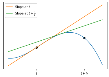
Runge-Kutta methods are derived from Taylor expansion(s) around intermediate point(s)¶

To derive the second-order Runge-Kutta method we:

1) estimate $x(t+h)$ using a Taylor expansion around $t+\frac{h}{2}$:

\begin{equation} x(t+h) = x(t+\frac{h}{2}) + \frac{h}{2}\left(\frac{\mathrm{d}x}{\mathrm{d}t}\right)_{t+\frac{h}{2}} + \frac{h^2}{8}\left(\frac{\mathrm{d}^2x}{\mathrm{d}t^2}\right)_{t+\frac{h}{2}}+\mathcal{O}(h^3) \end{equation}

2) estimate $x(t)$ using a Taylor expansion around $t-\frac{h}{2}$:

\begin{equation} x(t) = x(t+\frac{h}{2}) - \frac{h}{2}\left(\frac{\mathrm{d}x}{\mathrm{d}t}\right)_{t+\frac{h}{2}} + \frac{h^2}{8}\left(\frac{\mathrm{d}^2x}{\mathrm{d}t^2}\right)_{t+\frac{h}{2}}+\mathcal{O}(h^3) \end{equation}

3) Subtract Equation 2 from Equation 1 and re-arrange:

\begin{eqnarray} x(t+h) &=& x(t) + h\left(\frac{\mathrm{d}x}{\mathrm{d}t}\right))_{t+\frac{h}{2}}+\mathcal{O}(h^3) \\ x(t+h) &=& x(t) + hf(x(t+\frac{h}{2}),t+\frac{h}{2})+\mathcal{O}(h^3) \end{eqnarray}

Note: the $h^2$ term has completely disappeared, and the error term is now order $h^3$. We can say that this approximation is now accurate to order $h^2$.

The problem is that this requires knowledge of $x(t+\frac{h}{2})$ which we don't currently have. We can however estimate this using the Euler method!

\begin{equation} x(t+\frac{h}{2}) = x(t) + \frac{h}{2}f(x,t). \end{equation}

Substituting this into Equation 3 above, we can write the method for a single step as follows:

\begin{eqnarray} k_1 &=& hf(x,t) \\ k_2 &=& hf(x+\frac{k_1}{2},t+\frac{h}{2})\\ x(t+h) &=& x(t) + k_2 \end{eqnarray}

See how $k_1$ is used to give an estimate for $x(t+\frac{h}{2})$ ($k_2$), which is then substituted into the third equation to give an estimate for $x(t+h)$.

Note: Higher orde Runge-Kutta methods can be derived in a similar way - by calculating the Taylor series around various points and then taking a linear combination of the resulting expansions. As we increase the number of intermediate points, we increase the accuracy of the method. The downside is that the equations get increasingly complicated.

Keypoints:

The Runge-Kutta method is more accurate than Euler's method and runs just as fast
Runge-Kutta methods are derived from Taylor expansion(s) around intermediate point(s)
Runge-Kutta methods can be applied using the Python skills we have developed
We can easily compare our various models using the matplotlib plotting library